Until now, the main problem that we tried to solve was image classification, assigning one label to input image from the fixed set of categories. In the rest of this lecture, we try to give an overall view of other computer vision problems.
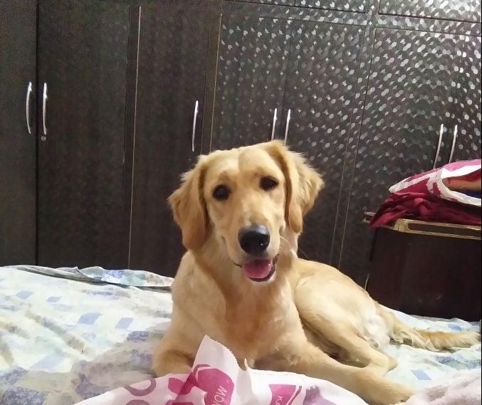
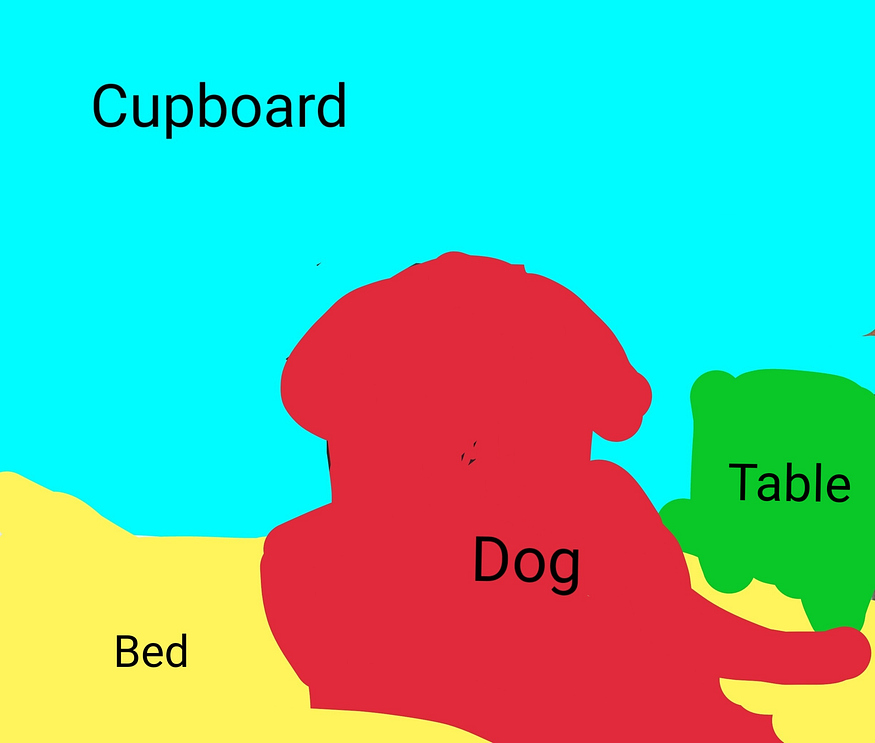
In semantic segmentation, we go one step forward and try to classify each pixel of an image instead of the input image as a whole.
❗Developing training data for semantic segmentation is too expensive.
The first idea to tackle this problem may be to use the sliding-window technic. Choose a small window, then move the window on the image and try to classify the center pixel of the window. But this method is not practical because it's very computationally expensive. Also, many computations are done that are redundant and could be shared.
The second idea is to design a big fully connected convolutional network that does predictions for each pixel at once. In this method, we preserve input image resolution in the whole network. preserving input image resolution in the whole network is expensive and could be problematic.
The last and commonly used idea is based on the previous one. But instead of preserving image resolution in the whole network, down-sampling and up-sampling are done. Down-sampling is done by usual convolutional layers and building the feature map. The new and unfamiliar part of the network is deconvolution layers that do up-sampling and produce classification scores for each pixel from the feature map.
We briefly explain some commonly used layers for up-sampling.
$$ \begin{bmatrix} 1 & 2\\ 3 & 4 \end{bmatrix} \to \begin{bmatrix} 1 & 1 & 2 & 2\\ 1 & 1 & 2 & 2\\ 3 & 3 & 4 & 4\\ 3 & 3 & 4 & 4\\ \end{bmatrix} $$
$$ \begin{bmatrix} 1 & 2\\ 3 & 4 \end{bmatrix} \to \begin{bmatrix} 1 & 0 & 2 & 0\\ 0 & 0 & 0 & 0\\ 3 & 0 & 4 & 0\\ 0 & 0 & 0 & 0\\ \end{bmatrix} $$
Max Unpooling is an improvement on the Bed of Nails layer. Most of the time, down-sampling and Up-sampling are done by symmetric networks that convolution and deconvolution parts are reflections of each other. So in max-pooling layers, the network remembers the location of the maximum element in each pool, and when arriving at the corresponding max-unpooling layers, input elements of the layer get laid in the remembered position of the bigger matrix.
$$ \begin{bmatrix} 1 & 3 & 2 & *7\\ 4 & *6 & 5 & 3\\ *4 & 2 & 3 & *5\\ 1 & 2 & 0 & 1\\ \end{bmatrix} \to \begin{bmatrix} 6 & 7\\ 4 & 5 \end{bmatrix} \to ... \to \begin{bmatrix} 1 & 2\\ 3 & 4 \end{bmatrix} \to \begin{bmatrix} 0 & 0 & 0 & *2\\ 0 & *1 & 0 & 0\\ *3 & 0 & 0 & *4\\ 0 & 0 & 0 & 0\\ \end{bmatrix} $$
The previous layers for up-sampling don't have any learnable parameters. But transpose convolution tried to be like the inverse of the convolution operation and has a kernel as a learnable parameter.
A general explanation of transpose convolution: