The vanilla neural network only could process input with fixed-length and produce fixed-length output. In RNN, we have a directed cycle between units (like state machines), allowing us to save some internal states from the input. This feature will enable us to process data with a dynamic length of input and output. Image captioning is an example of a one-to-many network, and machine translation is an example of a many-to-many network.

The recurrence formula is written below. The same set of parameters are used for every time step.
$$ h_t=f_W(h_{t-1},x_t) $$
A vanilla example for RNN.
$$ h_t = \tanh(W_{hh}h_{t-1}+W_{xh}x_t)\\y_t=W_{hy}h_t $$
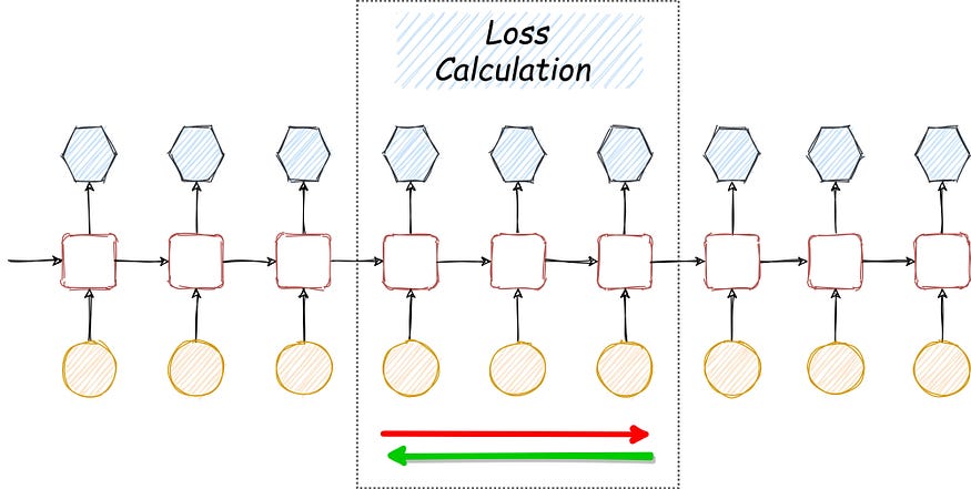
The Computational graph for many-to-many RNN is drawn. The overall loss is the sum of losses for each time step. Also, the gradient with respect to $W$ should be the sum of individual per time step gradients with respect to $W$.

Calculating the gradient for the whole sequence could be time-consuming and computationally expensive. To solve this problem, we use a similar trick as used in SGD. Instead of calculating the gradient for the whole sequence, we break the sequence into smaller chunks and update each chunk individually.

Truncate loss calculation